The Sticker Collector's Problem

An open box of Panini 2026 World Cup stickers with rows of packets inside, and a spread of opened stickers in front showing many duplicates of Mbappé, Messi, Haaland, Yamal and Ronaldo.

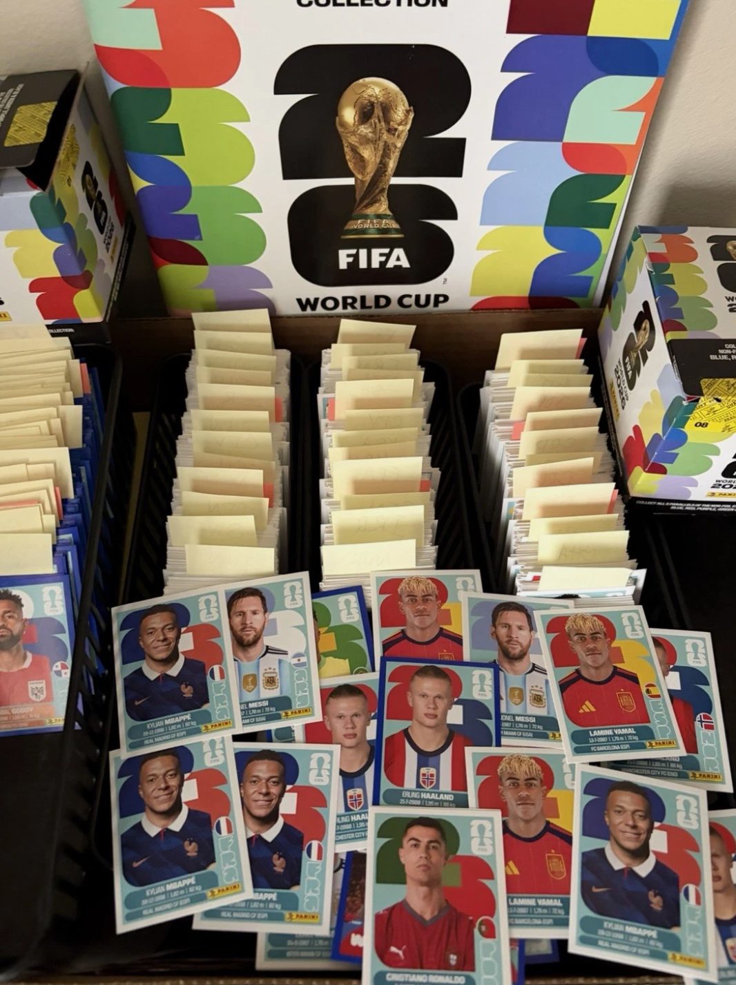
I’ve collected Panini World Cup stickers for as long as I’ve watched the World Cup. For a football fan, the album is part of the build-up to the tournament: the squads, the badges, the unfamiliar names, and the slow work of filling the pages before the first match.

This year is no different, except that the album is bigger than ever. The 2026 World Cup has expanded to 48 teams, and the sticker set has grown with it. The full album now has 980 stickers, which changes the economics of collecting it. A bigger album doesn’t just mean buying a few more packets. It makes the difficult part of the album longer and more expensive.

That difficult part usually comes near the end. You may only need 12 more stickers, but when you buy another packet, you find that all seven are duplicates. Buy another packet and you get much the same result. It’s easy to suspect that perhaps some stickers are being rationed, but the same thing can happen even when every sticker is printed in equal numbers.

For a 980-sticker album, completing the set by buying random packets takes about 7,300 stickers on average. That’s a little over 1,000 seven-sticker packets. At $1 a packet, the expected cost is about $1,000 to fill 980 slots. You buy more than seven albums’ worth of stickers, and most of them end up as duplicates.

This is an old probability problem in sticker-album form. Mathematicians call it the coupon collector’s problem: how long does it take to collect a complete set when the items arrive randomly, one at a time? Replace the coupons with World Cup stickers and the same logic applies.

The math also points to a better buying strategy. Random packets are worth it early in the process and much less useful near the end. The main question is when to switch.

Open Table of contents

Every new sticker is harder than the last
Your rare sticker isn’t actually rare
When the rarity is real: McDonald’s Monopoly
A collector is really a buyer
Trading is the cheapest strategy
The recipe: cheap early, precise late
Under the hood
What to do with all this

Every new sticker is harder than the last

Let’s start with the question that matters when you open a packet: will I get one of the stickers I’m missing?

To work that out, it helps to look at the stickers inside the packet one at a time. Suppose the album has $N$ spaces and you have already filled $k$ of them. A new sticker is equally likely to be any of the $N$ stickers in the set, so the chance that it lands on one of the $k$ spaces you’ve already filled is $k/N$ . In other words, the duplicate rate is just how full your album is.

A half-full album gives you a duplicate about half the time. A 90 percent full album gives you a duplicate about 90 percent of the time, so by that point most packets won’t help much.

Another way to say the same thing is that, if the album is fraction $f$ complete, a random sticker is new with probability $1-f$ . So the expected number of stickers you need to open before finding the next new one is:

$\frac{1}{1-f}.$

Show the math: why this formula works

Write $p = 1-f$ for the chance that a given sticker is new, and let $m$ be the average number of openings until the first new one.

Look at the very first opening. With probability $p$ it’s new, and you’re done after one opening. With probability $1-p$ it’s a duplicate: you’ve used one opening and you’re right back where you started, still facing an average of $m$ more. Putting those two cases together:

$m = 1 + (1-p)\,m.$

Solving for $m$ gives $p\,m = 1$ , so

$m = \frac{1}{p} = \frac{1}{1-f}.$

At 50 percent complete, you need about two openings for each new sticker. At 90 percent complete, you need about 10. At 99 percent complete, you need about 100.

With one slot left in a 980-sticker album, the chance that any given sticker fills it is $1/980$ . The expected wait for that final sticker is therefore 980 openings, or about 140 packets, just to fill one remaining space.

If you add those waits together, from the first sticker to the last one, you get:

$\frac{N}{N} + \frac{N}{N-1} + \frac{N}{N-2} + \cdots + \frac{N}{1} = N\left(\frac{1}{1} + \frac{1}{2} + \cdots + \frac{1}{N}\right).$

The sum in brackets is the harmonic series: $1 + \tfrac12 + \tfrac13 + \cdots$ , stopped at the $N$ -th term. It grows slowly, roughly like $\ln N + 0.58$ , where the 0.58 is the Euler-Mascheroni constant. For a 980-sticker album, the formula gives about 7,300 stickers, which is the number we started with.

These waits are independent of each other: once you hold a given number of stickers, how long you wait for the next new one depends only on how full the album is, not on which stickers you happened to get or how long the earlier waits took. So the expected total is just the sum of the expected waits.

Show the math: why those waits add up

Suppose you already own $k$ of the $N$ stickers. The next sticker you open is new with probability $\frac{N-k}{N}$ , so by the rule from the box above, the average wait for it is the reciprocal, $\frac{N}{N-k}$ .

The total wait to finish is just these added up, from your first new sticker ( $k=0$ ) to your last ( $k=N-1$ ):

$\frac{N}{N} + \frac{N}{N-1} + \cdots + \frac{N}{1} = N\left(1 + \frac{1}{2} + \cdots + \frac{1}{N}\right).$

That bracket is the harmonic sum, written $H_N$ , which is close to $\ln N + \gamma$ with $\gamma \approx 0.58$ . So the expected total is

$E[T] = N\,H_N \approx N(\ln N + \gamma).$

For $N = 980$ , this gives about $7{,}316$ stickers, or roughly $1{,}045$ seven-sticker packets.

Averages only tell part of the story. First, there’s a lot of variance. Two collectors can buy the same number of packets and end up in very different places, with a typical spread of well over 1,000 stickers around the average (there’s a derivation at the bottom). Second, most of the work comes near the end. The final one percent of the album, about 10 stickers in this example, takes a very large share of the total openings.

Collectors can therefore remember one sticker as especially hard to find, even when there’s nothing special about that sticker in the print run.

The same coupon collector’s problem shows up in plenty of other places: cereal-box toys, randomized rewards, and algorithms waiting to visit every state. Sticker albums are one everyday example.

Your rare sticker isn’t actually rare

Collectors often believe that some stickers are printed in smaller numbers. If you’ve opened hundreds of stickers and still haven’t found one particular badge or star player, “bad luck” can start to feel like an inadequate explanation.

But in a normal sticker album, bad luck plus a nearly full album is often enough.

Researchers have collected large samples of real stickers and checked whether some numbers appear less often than others. The answer has generally been no: the stickers appear to be close to evenly distributed, the same assumption we’ve been using. The feeling of rarity is real, but it doesn’t necessarily come from an uneven print run. It comes from the fact that, late in the album, every missing sticker is hard to find.

The birthday problem shows the same pattern. With only 23 people in a room, there’s already a better-than-even chance that two share a birthday. This is surprising because we tend to compare 23 people to 365 birthdays. The better comparison is all the possible pairs of people, and there are many of those. Collisions arrive earlier than most people expect.

Sticker albums are a slower version of the same thing. Even probabilities don’t prevent duplicates. They produce them. Long before the album looks close to full, duplicates start turning up; by the end, they dominate.

Show the math: the birthday problem in disguise

In the birthday problem, with $d$ equally likely birthdays, the chance that $n$ people all have distinct birthdays falls roughly like $e^{-n^2/2d}$ . This drops below one half once $n \approx 1.2\sqrt{d}$ . The same counting governs sticker collisions: with $N$ different stickers, the expected number of openings before your first duplicate is on the order of $\sqrt{N}$ , which for $N = 980$ is only about 30.

Uniform probabilities are enough to create a flood of duplicates, even without any hidden scarcity in the print run.

So the problem is probably not that Panini is holding back the sticker you need. Once you need only a few specific stickers, random buying becomes an expensive way to look for them.

When the rarity is real: McDonald’s Monopoly

McDonald’s Monopoly is a useful comparison because it looks like a collection game but works in almost the opposite way. It also shows what real scarcity looks like.

In a sticker album, the stickers are more or less equally likely. In McDonald’s Monopoly, some pieces are intentionally scarce. Each color group has common properties and one scarce piece. You can collect the common properties many times and still be no closer to winning if the rare piece never appears.

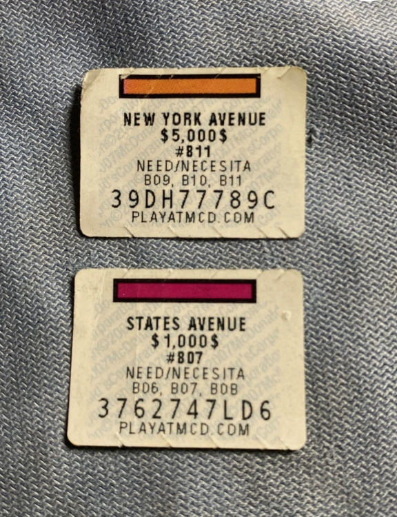
Two McDonald's Monopoly game pieces: an orange New York Avenue piece worth $5,000 (needs the set B09, B10, B11) and a magenta States Avenue piece worth $1,000 (needs B06, B07, B08). Both are common properties. — Two real game pieces. Each lists the properties you still need for the set, and in practice there is usually one piece that matters much more than the others.

This is still a coupon-collector problem, but with unequal probabilities. When the probabilities are uneven enough, the rarest item matters most, and the common pieces matter much less than the bottleneck piece.

That bottleneck was valuable enough to steal. For more than a decade, Jerome Jacobson, who worked in security for the promotion, stole rare winning pieces and passed them to a network of associates, rigging more than $20 million in prizes before the FBI caught on. The story later became the documentary McMillions.

The fraud worked for the same reason the promotion worked: the rare pieces were genuinely rare, while the common ones had little value on their own.

The two games work differently. In a sticker album, apparent rarity usually comes from even odds and a long tail. In McDonald’s Monopoly, rarity is designed into the system. With stickers, the print run is probably not the main issue; the bigger issue is how long you keep buying random packets.

A collector is really a buyer

It’s tempting to think of this as a question about luck. It’s better to think of it as a question about cost.

You can acquire stickers in two ways. You can buy packets at the store, or you can buy singles: the exact stickers you want, either from eBay or, for a limited window, on Panini’s official website. Packets are cheap per sticker but random. Singles are more expensive per sticker but exact. Early in the album, randomness is fine because almost everything is new. Late in the album, randomness is what makes packets expensive.

Call $c$ the cost of one sticker from a packet. If a seven-sticker packet costs $1, then $c$ is about 14 cents. Call $s$ the cost of buying one specific missing sticker as a single.

At completion level $f$ , only a fraction $1-f$ of opened stickers are new to you. So the effective cost of one useful new sticker from packets is:

$\frac{c}{1-f}.$

With an empty album, this is just the packet-sticker price. Half full, it doubles. At 90 percent full, a 14-cent sticker effectively costs about $1.40 for each new sticker you actually need. At 99 percent full, it’s about $14.

The marginal cost (the cost of the next new sticker) rises for packets as the album fills. For singles, it stays flat. The best time to switch is when those two costs meet:

$f^{*} = 1 - \frac{c}{s}.$

If a single costs twice as much as a packet sticker, the switch point is around 50 percent complete. If it costs four times as much, the switch point is around 75 percent. The more expensive singles are relative to packets, the longer packets remain worth buying.

Show the math: where the switch point comes from

Let the packet-sticker price be $c$ and the single price be $s$ . At completion level $f$ , a random sticker is new with probability $1-f$ , so the expected cost of one new sticker from packets is $\frac{c}{1-f}$ . Singles cost $s$ regardless.

Packets are cheaper while

$\frac{c}{1-f} < s \quad\Longleftrightarrow\quad f < 1 - \frac{c}{s}.$

Setting the two equal gives the switch level $f^{*} = 1 - \frac{c}{s}$ . Below it, packets are cheaper on the margin. Above it, singles are cheaper. If singles are no more expensive than packet stickers, so $s \le c$ , then $f^{*} \le 0$ and you should buy singles from the start.

The calculator below compares the two costs and works out the switch point for your own album. Set the album size, how many stickers you already have, the packet size, and the two prices. It marks where packets stop being the cheaper option and compares the cost of finishing from your current position under different strategies.

There’s one practical complication. Official single-ordering services often open late in the campaign and may cap how many stickers you can buy, so the formula isn’t always something you can follow exactly. It’s a benchmark for when packets have stopped being worth it, even if the market doesn’t yet let you fully act on it.

Trading is the cheapest strategy

Collecting alone makes the hobby more expensive, because all of your duplicates stay in your own pile.

A duplicate is nearly worthless to you, but it may be exactly what someone else needs. If you swap it for one of their duplicates that fills a gap in your album, both of you move forward and nobody buys another packet. In sticker form, this is the basic gains-from-trade argument.

This advantage grows in a group. Once several collectors pool their duplicates, the sticker that doesn’t appear in your packets is more likely to be sitting in somebody else’s spare pile. The larger the group, the more often that happens. Trading doesn’t eliminate the long tail, but it lowers the cost of dealing with it.

There are limits, since even a group that opens thousands of stickers can still be missing one last sticker. The final gap is still hard because the underlying probability problem hasn’t disappeared; it’s just been shared across more people. Trading is therefore most useful in the middle of the process, while the last few stickers are usually best acquired directly.

Your duplicates may also have resale value, especially during a popular campaign. Selling spares won’t change the whole economics of the album, but it can recover part of the cost. The real cost of the album is what you spend on packets and singles, minus what you recover through swaps and sales.

The recipe: cheap early, precise late

The practical strategy is to use random packets while they still make sense, and then move to more precise options.

In practice, that means three phases. The first is buying in bulk, because early on almost every sticker is useful. A box of packets, or a box that guarantees no repeats, clears the easy part of the album at a low effective price.

Then use trading to reduce the remaining gaps. Opening some additional packets can make sense if you want more swap material, but the main goal is no longer simply to buy volume. It’s to convert your duplicates into stickers you still need.

Once you’re down to the last few, the better option is to order the exact stickers you need. The end of the album is where packets are most expensive in effective terms and singles are most valuable.

The difference can be large. Buying packets all the way to the end costs a little over $1,000 on average in the 980-sticker example. A mixed strategy of bulk buying, trading, and a final singles order can finish the same album for far less, just by changing the order in which you buy things.

The benefit of treating the album as a spending problem is that you stop paying random prices for specific stickers.

Under the hood

A few more details for readers who want to understand the machinery behind the numbers.

How spread out is the total, really?

The expected total $N\,H_N$ tells you where the middle of the distribution sits, but not how far a typical collector lands from it. For that you want the variance.

The total wait is a sum of independent pieces, one for each new sticker, and for independent things the variances add. So the variance of the whole album is the sum of the variances of the individual waits. A geometric wait with success probability $p$ has variance $\frac{1-p}{p^2}$ , which for small $p$ is close to $\frac{1}{p^2}$ . In other words, the rarer the success, the bigger the variance, and it grows like the square of the average wait.

This is why the spread is dominated by the very end. When the album is nearly full, each new sticker has a small $p$ , a large average wait $\frac{1}{p}$ , and an even larger variance $\frac{1}{p^2}$ . The last handful of stickers contribute almost all of the uncertainty. Adding up those variances and keeping only the part that matters for a large album gives

$\operatorname{Var}(T) \approx \frac{\pi^2}{6}\,N^2.$

The $\frac{\pi^2}{6}$ comes from the sum $1 + \frac{1}{4} + \frac{1}{9} + \frac{1}{16} + \cdots$ , which the squared waits at the end of the album turn into. Taking the square root gives the standard deviation:

$\operatorname{sd}(T) \approx \frac{\pi}{\sqrt{6}}\,N \approx 1.28\,N.$

For a 980-sticker album that’s about 1,260 stickers, or roughly 180 packets. The average, $N\,H_N \approx 7{,}300$ , grows like $N\ln N$ , while the standard deviation grows only like $N$ , so in relative terms bigger albums are actually a little more predictable. In absolute terms the spread is still large: a standard deviation of 180 packets means two collectors following the same strategy can easily finish hundreds of dollars apart through luck alone.

Packs of seven, not one at a time

We’ve been treating openings as if stickers arrive one at a time. Real packets contain several stickers at once, usually seven, and modern packets often guarantee no repeats within a single packet. Both of these could, in principle, change the count.

They barely do. The only way a packet is worse than seven separate draws is if two stickers in the same packet would have been the same number, wasting one of them. But you’re drawing seven stickers from a set of nearly a thousand, so the chance that any two of them collide is tiny (this is the birthday problem again, with seven “people” and 980 “birthdays”). Almost every packet behaves like seven independent draws, so grouping them into sevens changes almost nothing.

The no-repeats guarantee pushes in the opposite direction: it removes the few within-packet collisions that would have happened, making a packet very slightly better than seven independent draws. Again the effect is small, because there were hardly any collisions to remove.

Both corrections are tiny and they point opposite ways, so the packet count stays close to the simple estimate of dividing the sticker total by seven: about $7{,}316 / 7$ , or 1,045 packets.

When stickers aren't equally likely (the Monopoly case)

So far every sticker has had the same chance, $1/N$ . McDonald’s Monopoly breaks that: sticker $i$ appears with its own probability $p_i$ , and some of those are deliberately tiny. When the probabilities are unequal, the expected time to collect the full set is given by an integral due to Flajolet and colleagues:

$E[T] = \int_{0}^{\infty}\!\left(1 - \prod_{i=1}^{N}\bigl(1 - e^{-p_i t}\bigr)\right)dt.$

The integral looks forbidding, but each piece has a plain meaning. Think of $t$ as how many stickers you’ve opened. For a single sticker $i$ , the chance you still haven’t seen it after $t$ openings decays like $e^{-p_i t}$ : a common sticker ( $p_i$ large) disappears from your “still missing” list quickly, while a rare one ( $p_i$ small) lingers. So $1 - e^{-p_i t}$ is the chance you have it by time $t$ , the product over all $i$ is the chance you have the complete set, and $1$ minus that product is the chance you’re still missing something. Adding up that “still missing” probability over all $t$ gives the expected time to finish.

The reason one item can dominate is in the decay rate. Suppose one sticker has a probability ten times smaller than the rest. Its $e^{-p_i t}$ term takes about ten times as long to shrink, so long after every common sticker is almost certainly collected, that single rare one is still holding the product down. The finishing time is set by whichever sticker is slowest to arrive, and with lopsided probabilities that’s almost always the rarest one. This is the formal version of the McDonald’s Monopoly point: once a single piece is much rarer than everything else, the whole game is really a wait for that one piece.

As $N$ grows, the finishing time also has a known limiting shape. After the right rescaling, it approaches a Gumbel distribution, the same extreme-value distribution that appears in problems governed by the maximum of many random quantities. This fits the sticker problem because finishing an album depends less on the average sticker than on the last one.

What to do with all this

The album probably isn’t rigged, and it doesn’t need to be. Fair odds are enough to make the ending slow and expensive, but they’re also something you can plan around: packets while most stickers are new, trades while your duplicates still have value to other people, and a direct order once randomness is doing almost nothing for you.

The next time a packet gives you seven duplicates, it may not mean the manufacturer is working against you. It may just mean you’ve been buying random packets for too long.