Why Are the Uyuni Salt Flats Hexagonal?

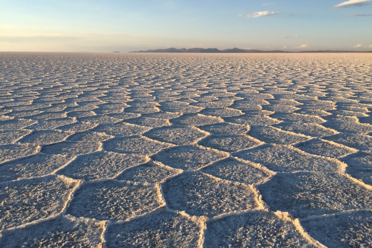
I recently got back from a trip to South America. I spent a few days in the Atacama Desert in northern Chile, and then crossed the border into Bolivia on a three-day overland tour that ended at the Salar de Uyuni. If you’ve ever wondered what the surface of another planet feels like underfoot, the Salar gets you most of the way there. Endless blinding white, a sky so blue it looks fake, and beneath your boots a perfectly tiled mosaic of hexagons stretching to the horizon.

That last detail is what I couldn’t stop thinking about. Why hexagons? Why so uniformly sized? Why does every salt flat on Earth do this same trick?

Table of contents

The obvious guess: it’s just mud cracks

The first theory that comes to mind (and one I heard on the tour) is that the salt crust dries out and cracks, much like mud does at the bottom of a drying puddle. You’ve seen those patterns: a wet flat surface contracts as it loses water, internal stress builds up, and eventually it splits along the lines of least resistance.

The problem is that mud cracks are messy. They form at all scales, from centimetres to half a metre across, and rarely settle into anything as orderly as a tiled hexagon. The Uyuni polygons are eerily consistent: roughly 1 to 2 metres across, the same dimensions you find in Death Valley’s Badwater Basin in California, in Botswana’s Sua Pan, and everywhere else this pattern appears on Earth. A drying-cracking story can’t explain that universality.

A second older hypothesis suggested that the salt crust grows so fast it buckles upward like a tile floor in summer, but it has the same defect: no fixed length scale. The real mechanism has to live somewhere else.

The real answer is underground

The real explanation was pinned down by Lasser et al. in Physical Review X in 2023, and the surprise is that the visible crust is only the last step. The mechanism lives in the porous, brine-saturated sediment underneath: a sponge-like layer of sand and silt soaked with salty groundwater.

Salt flats sit at the bottom of geographic sinks. Water flows in from the surrounding terrain, picks up dissolved salts, and the only way out is evaporation through the crust. Water leaves as vapour; salt stays behind. Over time this makes the brine just beneath the crust saltier, and therefore denser, than the fresher brine below.

That is the textbook setup for instability: dense fluid sitting above lighter fluid. Gravity wants the dense brine to sink and the lighter brine to rise, while viscosity in the sediment and salt diffusion resist the motion. When buoyancy wins, the subsurface overturns in slow convection. This is porous-media convection (or Rayleigh-Darcy convection), and it is what produces the pattern you see on top.

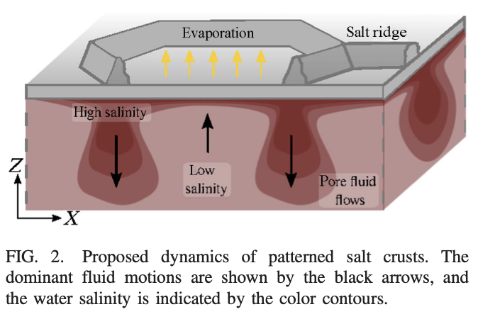
The salt ridges you see on the surface are essentially a residue map of the flow underneath. In the centre of each cell, relatively fresher brine rises toward the underside of the crust. Near the surface it spreads sideways, evaporation concentrates it, and by the time it reaches the edge of the cell it is saltier and denser. There it sinks back down.

Where two neighbouring cells meet, their sideways near-surface flows merge into a shared downwelling line. That persistent line of dense, salty brine feeds faster crystallisation above it, so the crust slowly builds upward into a ridge. The centres, fed by fresher upwelling brine, accumulate less salt and stay lower. The hexagons are not really a feature of the crust alone; they are the surface signature of fluid circulation below.

How the pattern grows

The hexagonal lattice doesn’t appear all at once. It assembles itself as convection cells nucleate at slightly different points and then reorganise into a shared network.

Just before the instability kicks in, the brine layer is uniform but on edge. Tiny random perturbations get amplified into distinct upwelling and downwelling zones. The important surface feature is not the exact path a parcel of brine takes, but the persistent network of downwelling sheets that forms where neighbouring circulation zones meet. Those downwelling sheets become the ridge template.

Mathematically this resembles a Voronoi tessellation: each cell owns the points closest to its centre. That is not a literal model of the brine. It is a geometric cartoon of the same kind of competition: neighbouring cells expand, meet, and share boundaries.

The animation below uses Lloyd-style relaxation as a drawing trick. Lloyd’s algorithm repeatedly recentres each cell and makes a Voronoi network more regular; it minimises a centroidal energy, not perimeter directly. But for roughly uniform cells on a plane, the endpoint is the same visual attractor: an evenly spaced, hexagon-dominated lattice. The Salar is not running Lloyd’s algorithm underground. The analogy is just a way to see how an irregular cell network can settle toward six-sided order.

This is the bridge between the fluid physics and the geometry. The convection underneath dictates that cells form. The Voronoi picture explains why neighbouring cells generate a polygon network. The relaxation step is only a visual analogy, but it captures the key geometric tendency: an initially irregular network becomes more evenly spaced and more hexagon-like.

Why hexagons, specifically?

From here on, the argument is geometric. Each individual convection cell, left in isolation, would prefer to be circular, because a circle minimises perimeter for a given area. But you can’t tile a plane with circles without leaving gaps. Once many cells start competing for the same surface area, they get packed together, and the question becomes: among shapes that do tile the plane regularly, which one has the lowest perimeter-to-area ratio?

There are only three regular tilings: triangles, squares, and hexagons. For a unit area:

The hexagon wins. The pattern generalises cleanly: a regular $n$-gon of unit area has perimeter

$P(n) = 2\sqrt{n \tan(\pi/n)}.$

Take the derivative and after a line of algebra the sign of $dP/dn$ reduces to whether $\sin(2\pi/n) < 2\pi/n$, which is just $\sin x < x$ for $x > 0$. True for every $n \geq 3$, so $P(n)$ is strictly decreasing: more sides means less perimeter per unit area. The circle is the $n \to \infty$ limit at $P = 2\sqrt{\pi} \approx 3.545$, the absolute optimum. But circles don’t tile, they leave gaps. Among regular shapes that do tile the plane (only $n = 3, 4, 6$), you take the one with the most sides: the hexagon.

That much has been known since Pappus of Alexandria around 320 AD. But Pappus’s argument only handles regular polygons with straight edges. Real cells in nature, the polygons on a salt flat, the bubbles in a foam, the cells in biological tissue, have boundaries that can bulge outward or curve inward. A wavy boundary could in principle enclose more area for less perimeter than any polygon. So does the hexagon really still win in the general case?

This is what Thomas Hales finally settled in 1999, in the result now called the honeycomb theorem. The statement: for any partition of the plane into regions of equal area, allowing arbitrary smooth curves as boundaries, the perimeter per unit cell is at least

$\sqrt[4]{12} \approx 3.7224,$

with equality only for the regular hexagonal tiling. As a sanity check, this matches the regular-hexagon formula:

$2\sqrt{6\tan(\pi/6)} \;=\; 2\sqrt{2\sqrt{3}} \;=\; 2\sqrt[4]{12}.$

L. Fejes Tóth had extended Pappus to all convex cells back in 1943. Hales removed the convexity assumption, which is the case that actually applies to nature, where cell boundaries are free to wave around.

Bees got there empirically long before Hales did, and they had an economic motive. A worker bee has to digest roughly eight units of honey to secrete one unit of wax, so wax is genuinely expensive in bee currency. Storing the most honey per unit of wax (read: maximum area per minimum perimeter) is a real pressure on the hive’s economy. The honeycomb’s hexagons are the same answer the salt flat arrives at by physics alone. Among shapes that can pack together to cover an area, even with curvy boundaries, the hexagon is the cheapest perimeter you can buy.

For the salt flat, the relevant “perimeter” is the network of shared downwelling fronts between cells. Shorter total boundary length is the cheaper way to pack equal-area circulation cells together. That does not mean every polygon becomes a perfect hexagon: real salt flats have boundary effects, finite-time growth, noise, pentagons, and heptagons. But the low-perimeter tendency explains why six-sided cells dominate.

Why about a metre across?

The size of the cells is set by the dimensionless Rayleigh-Darcy number, which governs convection in porous media:

$Ra = \frac{\Delta\rho \, g \, K \, L}{\mu \, D}$

Here Δρ is the density contrast between salty and fresher brine, $g$ is gravity, $K$ is the permeability of the sediment, $L$ is the depth of the convecting layer, $\mu$ is the brine’s dynamic viscosity, and $D$ is the salt diffusivity. Convection switches on once $Ra$ crosses a critical threshold (around $4\pi^2 \approx 39.5$ for the simplest case).

When you plug in realistic numbers for a typical salt flat, the fastest-growing instability lands at a length scale of roughly one to two metres. That is why playas with different chemistry and geology still end up with similar-looking polygons. The scale is not set by the size of the basin; it comes from the local balance between buoyancy, diffusion, viscosity, permeability, and evaporation-driven salinity gradients.

Compare this to a drying mud flat. Mud cracks, columnar basalt joints, frozen-ground polygons, and the cracking patterns on crocodile snouts all obey a simple rule: the spacing between cracks scales with the thickness of the cracking layer (Goehring & Morris, 2014). Thin mud cracks fine, thick basalt cracks into metre-scale columns, and the geometry of the layer sets the length scale; the underlying mechanism is mechanical, with stress building up in a layer as it dries or cools until it fractures.

Salt polygons break this rule. The crust thickness varies by orders of magnitude between sites, yet the polygons stay stubbornly one to two metres across everywhere. That is exactly why they puzzled scientists for so long: they look like cracks but obey none of the cracking-pattern rules. The length scale comes from the convection underneath, where the Rayleigh-Darcy number sets the scale from universal fluid properties rather than from local geometry. A salt flat looks like dried mud but is built on completely different physics. Lukas Goehring, who wrote the canonical Physics Today piece on layer-thickness cracking patterns, co-authored the Lasser paper a decade later that found salt polygons are the exception to his own rule.

Standing on the Salar

So when you’re out there squinting at the glare, you’re really standing on top of a very slow, very quiet plumbing system. Each hexagon under your boots is the top of a single convection cell that has been turning over for months, in a kind of geological breathing. The crust is just the visible top layer of a hidden fluid dynamics problem, and it happens to be one of the most universal pattern-forming mechanisms in physics.

It also explains why the Star Wars: The Last Jedi crew chose the Salar to film an alien battlefield. Whatever planet Crait was supposed to be, the physics underneath was Earth’s all along.

Further reading

• Lasser et al. Salt Polygons and Porous Media Convection. Physical Review X 13, 011025 (2023). arXiv:1902.03600
• Beaume, Goehring & Lasser. Hidden Fluid Dynamics of Dry Salt Lakes. Physics Today 77(4), 62 (2024).
• Goehring & Morris. Cracking mud, freezing dirt, and breaking rocks. Physics Today 67(11), 39-44 (2014). DOI: 10.1063/PT.3.2584
• Hales. The Honeycomb Conjecture. Discrete & Computational Geometry 25, 1 (2001). arXiv:math/9906042
• Buchanan, M. Why Death Valley Is Full of Polygons. Physics 16, 31 (2023). physics.aps.org/articles/v16/31
• ScienceNews. Here’s why the geometric patterns in salt flats worldwide look so similar. sciencenews.org/article/geometric-patterns-salt-flats-worldwide
• ScienceAlert. Salt Deserts Are Covered in Strange, Repeating Patterns. We’ve Finally Figured Out Why. sciencealert.com